RAI Exercise 1: Algorithmic Fairness ⚖️

Important information

This exercise is part of the RAI course (02517 - Responsible AI: Algorithmic Fairness and Explainability) at the Technical University of Denmark (DTU). You can find more details about the course here. This specific version is for the Fall 2024 semester.

If you have any questions related to this notebook, feel free to reach out to Nina Weng at ninwe@dtu.dk.

Credits:
We thank:

• NIH dataset team for collecting such dataset link to the paper;
• Authors from this paper for providing the splits;
• Memes generator webpage imgflip for all the excellent Memes template.

PART 1: Fairness assessment and Bias mitigation using Fairlearn

The goal of this exercise is to learn how to use Fairlearn to approach basic fairness assessments and apply post-processing bias mitigation methods.

Fairlearn is an open-source Python package originally developed by Microsoft Research. Since 2021, it has become completely community-driven. For more information about Fairlearn, you can visit this page).

Although Fairlearn is likely the most well-developed package targeting fairness issues, it has its limitations. The most notable limitation, that might need to be mentioned at very beginning for this exercise, is that Fairlearn is primarily designed for tabular data (this page under question: Does Fairlearn work for image and text data?). Therefore, when working with other types of data, such as image data, unexpected issues may arise. Fortunate enough, there are workarounds for most of these issues, which will be discussed later in this exercise.

While Fairlearn is a good resource and offers an easy approach for learning fairness concepts and handling lighter tasks, it may not be the best solution for researchers working extensively in this area. Keep that in mind :-)

🧠 Objective of this Exercise (PART 1)

By the end of this exercise, you should be able to:

• Assess fairness using Fairlearn with provided predictions/probabilities and target labels. This includes calculating metrics, generating ROC curves, and interpreting their meaning.
• Apply post-processing bias mitigation techniques using Fairlearn, and clearly understand and explain the outcomes.

1. Dataset: Chest X-ray and lung/heart related disease

In this exercise, we will use a chest X-ray dataset and a basic deep learning model as the setup. It requires the following:

• Download the dataset/metadata/pretrained ResNet model. Note that in this exercise, we only use part of the data, and details are listed below. The full dataset can be found here. (For students in the class, you can find a download link on DTU Learn. For those not in the class, you can find the pre-processing scripts in this repository.)
• After downloading the materials, put the NIH_train_val_test_rs0_f50.csv under ./datafiles/; and nih_pneumothorax.pth under ./pretrained_model/.
• Prepare your virtual environment: #TODO

Chest xray samples

We use NIH chest xray dataset in this exercise. Let’s take a closer look at the dataset.

This dataset contains 108,948 images from 32,717 patients, each labeled with one of 14 types of lung or heart-related diseases/symptoms. For detailed information on each disease, you can find explanations here.

For simplicity, we will use only one sample per patient and preprocess the images to a size of 224x224. Both the dataset and the metadata (in CSV format) are available. The dataset split is also specified in the metadata under the column 'split'.

Note: The split was designed for a different task, which required a larger test set than usual. As a result (as you’ll notice), the test set is relatively large (around 8k for training, 2k for validation, and 8k for testing). If you find that the mitigation or prediction process takes too long, feel free to downsample the test set. Just ensure you validate that the proportions of samples across different sensitive groups and disease labels remain roughly consistent with the original test set.

import os
import matplotlib.pyplot as plt
import matplotlib.image as mpimg
import pandas as pd
import seaborn as sns
sns.set_theme(style="whitegrid")
import torch

from tqdm import tqdm
from sklearn.metrics import accuracy_score
from fairlearn.metrics import MetricFrame, selection_rate,false_positive_rate,true_positive_rate,false_negative_rate,true_negative_rate


#
from train.model import ResNet
from train.prediction import validate
from analysis.plot import plot_roc_simple
from analysis.tools import from_loader_to_tensor

#TODO: change this to your data directory
datadir = '/work3/ninwe/dataset/'

Let us take a look of some samples, with filter query.

dataset_pth = datadir + '/NIH_part/'
dataset_pth = datadir + '/NIH/preproc_224x224/'
metadata_csv ='./datafiles/NIH_train_val_test_rs0_f50.csv'
metadata = pd.read_csv(metadata_csv)

# display(metadata.head(5))

# randomly choose some samples from PAD-UFES-20
def show_random_images(datadir,metadata,seed=None,filter_str=None,num_sample=5):
    fig = plt.figure(figsize=(num_sample*3, 3),dpi=200)
    files = os.listdir(datadir)
    if filter_str:
        metadata = metadata.query(filter_str)
        # display(metadata.head(5))
    if seed is not None:
        random_sample = metadata.sample(n=num_sample, random_state=seed)
    else: random_sample = metadata.sample(n=num_sample)
    
    for i in range(len(random_sample)):
        row = random_sample.iloc[i]
        disease = row['Pneumothorax']
        sex = row['Patient Gender']

        img = mpimg.imread(datadir + row['Image Index'])
        ax = fig.add_subplot(1, len(random_sample), i + 1)
        # add diagnosis as subtitle
        ax.set_title(f'{disease=},{sex=}')
        ax.imshow(img, cmap='gray')
        ax.axis('off')
    plt.suptitle(f'{filter_str}')
    plt.show()

show_random_images(dataset_pth,metadata=metadata,seed=42,filter_str='Pneumothorax==1 and `Patient Gender`=="F"',num_sample=5)
show_random_images(dataset_pth,metadata=metadata,seed=42,filter_str='Pneumothorax==1 and `Patient Gender`=="M"',num_sample=5)

Basic statistics

We can also take a look at the distribution of some sensitive attributes:

def plot_distribution_by_value(metadata, column_name):
    if isinstance(column_name, str):
        nan_count = metadata[column_name].isna().sum()
        nan_series = pd.Series([nan_count], index=['NaN'])
        counts_ = metadata[column_name].value_counts().sort_index()
        counts_with_nan = pd.concat([counts_, nan_series])

        counts_with_nan.plot(kind='bar',title='Distribution of {}'.format(column_name))
        plt.ylabel('count')
    elif isinstance(column_name, list):
        fig, axes = plt.subplots( 1, len(column_name), figsize=( len(column_name)*4,3),dpi=200)
        for i,col in enumerate(column_name):
            nan_count = metadata[col].isna().sum()
            nan_series = pd.Series([nan_count], index=['NaN'])
            counts_ = metadata[col].value_counts().sort_index()
            counts_with_nan = pd.concat([counts_, nan_series])

            counts_with_nan.plot(kind='bar',title='Distribution of {}'.format(col),ax=axes[i])
            axes[i].set_ylabel('count')
    plt.tight_layout()
    plt.show()

metadata['age_range'] = pd.cut(metadata['Patient Age'], bins=[0,10,20,30,40,50,60,70,80,90,100], right=False)
plot_distribution_by_value(metadata, ['age_range','Patient Gender'])

You may have noticed that, for this specific split, we maintain an equal number of male and female samples. This balance is consistent across all three splits: training, validation, and testing.

📃 Further Reading:

If you're interested, here are some studies that explore potential biases and confounders in chest xray datasets:

• Lauren Oakden-Rayner: Exploring the ChestXray14 dataset: problems
• Amelia Jiménez-Sánchez et al.: Detecting Shortcuts in Medical Images -- A Case Study in Chest X-rays
• Judy Wawira Gichoya et al.: AI recognition of patient race in medical imaging: a modelling study00063-2/fulltext)

2. Fairness assessment

Recap of Key Concepts:

In th class, we have learned:

• The three key criteria for fairness assessment. What are they?
• Evaluation metrics corresponding to each criterion.
• ROC curves.

For this exercise, we’ve provided a pre-trained ResNet classifier for Part 1, where the disease label is Pneumothorax and the sensitive attribute is sex (in metadata, you can get the binarized sex label from column sex label, where 0 represents female and 1 represents male). However, feel free to train your own model if you'd like.

Load pretrained model

# load the pretrained model
device = 'cuda' if torch.cuda.is_available() else 'cpu'
print(' device:', device)

ds_name = 'NIH'

# load the model
lr=1e-6
pretrained = True
model_scale = '18'
num_epochs =20
img_size = (1, 224, 224)

classifier = ResNet(num_classes=1, lr=lr, pretrained=pretrained, model_scale=model_scale, in_channel=img_size[0])
classifier.load_state_dict(torch.load('./pretrained_model/nih_pneumothorax.pth'))
classifier.to(device)

classifier.eval()

 device: cuda

/work3/ninwe/miniconda3/envs/rai_fairness/lib/python3.9/site-packages/torchvision/models/_utils.py:208: UserWarning: The parameter 'pretrained' is deprecated since 0.13 and may be removed in the future, please use 'weights' instead.
  warnings.warn(
/work3/ninwe/miniconda3/envs/rai_fairness/lib/python3.9/site-packages/torchvision/models/_utils.py:223: UserWarning: Arguments other than a weight enum or `None` for 'weights' are deprecated since 0.13 and may be removed in the future. The current behavior is equivalent to passing `weights=ResNet18_Weights.IMAGENET1K_V1`. You can also use `weights=ResNet18_Weights.DEFAULT` to get the most up-to-date weights.
  warnings.warn(msg)

ResNet(
  (model): ResNet(
    (conv1): Conv2d(1, 64, kernel_size=(7, 7), stride=(2, 2), padding=(3, 3), bias=False)
    (bn1): BatchNorm2d(64, eps=1e-05, momentum=0.1, affine=True, track_running_stats=True)
    (relu): ReLU(inplace=True)
    (maxpool): MaxPool2d(kernel_size=3, stride=2, padding=1, dilation=1, ceil_mode=False)
    (layer1): Sequential(
      (0): BasicBlock(
        (conv1): Conv2d(64, 64, kernel_size=(3, 3), stride=(1, 1), padding=(1, 1), bias=False)
        (bn1): BatchNorm2d(64, eps=1e-05, momentum=0.1, affine=True, track_running_stats=True)
        (relu): ReLU(inplace=True)
        (conv2): Conv2d(64, 64, kernel_size=(3, 3), stride=(1, 1), padding=(1, 1), bias=False)
        (bn2): BatchNorm2d(64, eps=1e-05, momentum=0.1, affine=True, track_running_stats=True)
      )
      (1): BasicBlock(
        (conv1): Conv2d(64, 64, kernel_size=(3, 3), stride=(1, 1), padding=(1, 1), bias=False)
        (bn1): BatchNorm2d(64, eps=1e-05, momentum=0.1, affine=True, track_running_stats=True)
        (relu): ReLU(inplace=True)
        (conv2): Conv2d(64, 64, kernel_size=(3, 3), stride=(1, 1), padding=(1, 1), bias=False)
        (bn2): BatchNorm2d(64, eps=1e-05, momentum=0.1, affine=True, track_running_stats=True)
      )
    )
    (layer2): Sequential(
      (0): BasicBlock(
        (conv1): Conv2d(64, 128, kernel_size=(3, 3), stride=(2, 2), padding=(1, 1), bias=False)
        (bn1): BatchNorm2d(128, eps=1e-05, momentum=0.1, affine=True, track_running_stats=True)
        (relu): ReLU(inplace=True)
        (conv2): Conv2d(128, 128, kernel_size=(3, 3), stride=(1, 1), padding=(1, 1), bias=False)
        (bn2): BatchNorm2d(128, eps=1e-05, momentum=0.1, affine=True, track_running_stats=True)
        (downsample): Sequential(
          (0): Conv2d(64, 128, kernel_size=(1, 1), stride=(2, 2), bias=False)
          (1): BatchNorm2d(128, eps=1e-05, momentum=0.1, affine=True, track_running_stats=True)
        )
      )
      (1): BasicBlock(
        (conv1): Conv2d(128, 128, kernel_size=(3, 3), stride=(1, 1), padding=(1, 1), bias=False)
        (bn1): BatchNorm2d(128, eps=1e-05, momentum=0.1, affine=True, track_running_stats=True)
        (relu): ReLU(inplace=True)
        (conv2): Conv2d(128, 128, kernel_size=(3, 3), stride=(1, 1), padding=(1, 1), bias=False)
        (bn2): BatchNorm2d(128, eps=1e-05, momentum=0.1, affine=True, track_running_stats=True)
      )
    )
    (layer3): Sequential(
      (0): BasicBlock(
        (conv1): Conv2d(128, 256, kernel_size=(3, 3), stride=(2, 2), padding=(1, 1), bias=False)
        (bn1): BatchNorm2d(256, eps=1e-05, momentum=0.1, affine=True, track_running_stats=True)
        (relu): ReLU(inplace=True)
        (conv2): Conv2d(256, 256, kernel_size=(3, 3), stride=(1, 1), padding=(1, 1), bias=False)
        (bn2): BatchNorm2d(256, eps=1e-05, momentum=0.1, affine=True, track_running_stats=True)
        (downsample): Sequential(
          (0): Conv2d(128, 256, kernel_size=(1, 1), stride=(2, 2), bias=False)
          (1): BatchNorm2d(256, eps=1e-05, momentum=0.1, affine=True, track_running_stats=True)
        )
      )
      (1): BasicBlock(
        (conv1): Conv2d(256, 256, kernel_size=(3, 3), stride=(1, 1), padding=(1, 1), bias=False)
        (bn1): BatchNorm2d(256, eps=1e-05, momentum=0.1, affine=True, track_running_stats=True)
        (relu): ReLU(inplace=True)
        (conv2): Conv2d(256, 256, kernel_size=(3, 3), stride=(1, 1), padding=(1, 1), bias=False)
        (bn2): BatchNorm2d(256, eps=1e-05, momentum=0.1, affine=True, track_running_stats=True)
      )
    )
    (layer4): Sequential(
      (0): BasicBlock(
        (conv1): Conv2d(256, 512, kernel_size=(3, 3), stride=(2, 2), padding=(1, 1), bias=False)
        (bn1): BatchNorm2d(512, eps=1e-05, momentum=0.1, affine=True, track_running_stats=True)
        (relu): ReLU(inplace=True)
        (conv2): Conv2d(512, 512, kernel_size=(3, 3), stride=(1, 1), padding=(1, 1), bias=False)
        (bn2): BatchNorm2d(512, eps=1e-05, momentum=0.1, affine=True, track_running_stats=True)
        (downsample): Sequential(
          (0): Conv2d(256, 512, kernel_size=(1, 1), stride=(2, 2), bias=False)
          (1): BatchNorm2d(512, eps=1e-05, momentum=0.1, affine=True, track_running_stats=True)
        )
      )
      (1): BasicBlock(
        (conv1): Conv2d(512, 512, kernel_size=(3, 3), stride=(1, 1), padding=(1, 1), bias=False)
        (bn1): BatchNorm2d(512, eps=1e-05, momentum=0.1, affine=True, track_running_stats=True)
        (relu): ReLU(inplace=True)
        (conv2): Conv2d(512, 512, kernel_size=(3, 3), stride=(1, 1), padding=(1, 1), bias=False)
        (bn2): BatchNorm2d(512, eps=1e-05, momentum=0.1, affine=True, track_running_stats=True)
      )
    )
    (avgpool): AdaptiveAvgPool2d(output_size=(1, 1))
    (fc): Linear(in_features=512, out_features=1, bias=True)
  )
  (loss_fn): BCEWithLogitsLoss()
  (accu_func): BinaryAccuracy()
  (auroc_func): BinaryAUROC()
)

Load test and validation data

save_model_at = './pretrained_models/'

img_size = (1,224,224)
batch_size = 16

csv_pth = './datafiles/NIH_train_val_test_rs0_f50.csv' if ds_name == 'NIH' else None

disease_label = 'Pneumothorax' 
sensitive_label = 'sex'
augmentation = False

from train.train_chestxray import create_datasets

train_dataset, val_dataset, test_dataset = create_datasets(dataset_pth, 
                                                               ds_name,
                                                               csv_pth, 
                                                               image_size=img_size, 
                                                               device=device,
                                                               disease_label = disease_label,
                                                               sensitive_label = sensitive_label,
                                                               augmentation=augmentation)
# train_loader = torch.utils.data.DataLoader(train_dataset, batch_size=batch_size, shuffle=True) # we dont need it here
val_loader = torch.utils.data.DataLoader(val_dataset, batch_size=batch_size, shuffle=False)
test_loader = torch.utils.data.DataLoader(test_dataset, batch_size=batch_size, shuffle=False)

Loading Data: 100%|██████████| 8458/8458 [00:00<00:00, 14572.82it/s]
Loading Data: 100%|██████████| 1409/1409 [00:00<00:00, 22418.20it/s]
Loading Data: 100%|██████████| 8459/8459 [00:00<00:00, 22569.23it/s]

Predict the results for test set

test_lab, test_pred, test_prob, test_a= validate(classifier, test_loader, device=device)

100%|██████████| 529/529 [00:35<00:00, 15.07it/s]

val_loss=1.2348 val_acc=0.8094 val_auroc=0.7726

Assess fairness using Fairlearn

A simple example first

Fairlearn provides the fairlearn.metrics.MetricFrame class to help with this quantification.

Given:

y_true = [0, 1, 1, 1, 1, 0, 1, 0, 1, 0, 0, 0, 1, 1, 1, 1, 1, 1]
y_pred = [0, 0, 1, 0, 1, 1, 1, 0, 0, 1, 1, 1, 1, 0, 0, 1, 1, 0]
sf_data = ['b', 'b', 'a', 'b', 'b', 'c', 'c', 'c', 'a',
           'a', 'c', 'a', 'b', 'c', 'c', 'b', 'c', 'c']

Try:

• measure: recall, selection rate and false positive rate for each group;
• plot the above result out; (Hint)
• measure the difference in eqaulized odd between different groups;

Hint: The documentation page of MetricFrame

Now measure the fairness metrics for our data

mf = MetricFrame(metrics={'accuracy': accuracy_score,
                            'selection_rate': selection_rate,
                            'false_positive_rate': false_positive_rate,
                            'true_positive_rate': true_positive_rate,
                            'true_negative_rate': true_negative_rate,
                         },
                 y_true=test_lab,
                 y_pred=test_pred,
                 sensitive_features=test_a)

print("Test set fairness metrics (before mitigation):")
print(mf.by_group)

Test set fairness metrics (before mitigation):
                     accuracy  selection_rate  false_positive_rate  \
sensitive_feature_0                                                  
0.0                  0.769213        0.244029             0.222028   
1.0                  0.849645        0.155083             0.137463   

                     true_positive_rate  true_negative_rate  
sensitive_feature_0                                          
0.0                            0.619658            0.777972  
1.0                            0.556180            0.862537  

Draw the ROC curve

plot_roc_simple(test_lab, test_prob, test_a, test_pred,
        sensitive_attribute_name = 'sex',
        )

💥 Exercise and discusssion:

• What do you see from the metrics and the ROC curve?
• Try to measure and desribe the fairness wrt the 3 creterias we learned from class

3. Bias mitigation using Fairlearn

Recall from the class

• what kinds of mitigation methods have we learned?

In this exercise, we will try to use the one pf the post-preprocessing bias mitiagtion method Fairlearn provided: Threshold Optimization, to implement the bias mitigation steps.

The theory of Threshold Optimization

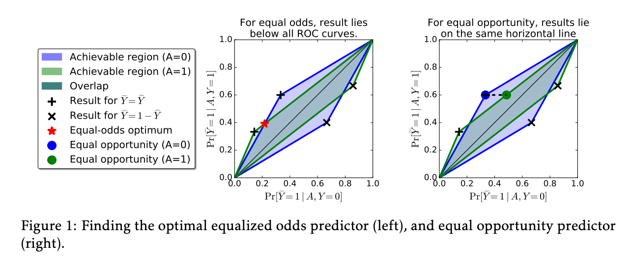
The idea could be simply visualized as below (figure from the original paper):

Where blue/green represent two sensitive groups, any points in the overlapping region meet the requirement of equalized odds:

$$ \gamma_0(\hat{Y}) = \gamma_1(\hat{Y}), $$

where

$$ \gamma_a (\hat{Y}) = \left(Pr(\hat{Y} = 1 | A = a, Y = 0), Pr(\hat{Y} = 1 | A = a, Y=1)\right). $$

The goal of the threshold optimizer is to find the point in the overlapping region that optimizes the objective function, such as balanced accuracy.

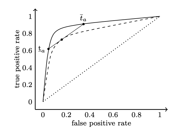
To achieve this, randomization is introduced. The idea is starightforward: any point under the ROC curve can be estimated by weighting two points on the ROC curve (which could be achieved by simply thresholding); or in another word, a new decision threshold $T_a$ can be a randomized mixture of two decision thresholds $\underline{t}_a$ and $\overline{t}_a$.

(See the figure below, which is from this paper).

📃 Further Reading:

• Fairlearn ThresholdOptimizier page.
• The original paper (See section 3): Equality of opportunity in supervised learning.

🪄 Trick: A fake classifier class

Fairlearn has some limitations when implementing the ThresholdOptimizer method. To work around these issues, a fake classifier is provided to bypass minor problems. If you use the provided classifier, this fake class should work just as well.

However, if you're curious about what went wrong or want to use your own classifier, please read below:

• Problem 1: estimator in ThresholdOptimizer only accepts 2D input (tabular data). This doesn’t make sense for post-processing mitigation methods, as the only relevant aspect here is the prediction scores from the test set. The classifier itself and the input data are irrelevant when optimizing the threshold.

• Problem 2: The prefit parameter checks whether the model has been fitted in a simplistic way, leading to errors. You can read more about this fit check function here.

• Problem 3: It requires the prediction function to return scores for both classes in binary classification. This might be an issue if your classifier only provides the probability for class 1.

How we solve this: We create a fake classifier that accepts 2D input and reshapes it back to the original image size before feeding it into the prediction function. We trick the fit check by defining a fake variable and manually modify the output of the prediction function to include both classes if it only returns the probability for class 1.

Note: If you trained your own classifier, you will need to implement a custom fake classifier yourself.

from sklearn.base import BaseEstimator, ClassifierMixin

class FakeClassifierInput2D(BaseEstimator,ClassifierMixin):
    '''
    Fake classifier that takes 2D input, with pre-trained model that does not take 2D input data
    '''
    def __init__(self,model, img_size):
        self.model = model
        self.img_size = img_size
        self.input_from_2D_func = lambda x: torch.reshape(x,(-1,)+self.img_size)
        # self.input_from_2D_func = input_from_2D_func
        self.fit_ = True # fake the check_fit function inside the fairlearn library

    def fit(self, X, y):
        # Do not need to fit
        return

    def predict(self, X_2D, ):
        assert len(X_2D.shape) == 2
        X = self.input_from_2D_func(X_2D)
        return self.model.predict(X)
    
    def predict_proba(self, X_2D):
        X = self.input_from_2D_func(X_2D)
        return self.model.predict_proba(X)
    

Optimize on validation set

X_test, y_test, a_test = from_loader_to_tensor(test_loader,device)
X_val, y_val, a_val = from_loader_to_tensor(val_loader,device)

X_test_2D = torch.reshape(X_test,(X_test.shape[0],-1))

100%|██████████| 529/529 [00:24<00:00, 21.88it/s]

X.shape=torch.Size([8459, 1, 224, 224]), y.shape=torch.Size([8459]), a.shape=torch.Size([8459])

100%|██████████| 89/89 [00:04<00:00, 22.11it/s]

X.shape=torch.Size([1409, 1, 224, 224]), y.shape=torch.Size([1409]), a.shape=torch.Size([1409])

classifier_fake = FakeClassifierInput2D(model=classifier.to('cpu'),
                                       img_size = img_size,)

from fairlearn.postprocessing import ThresholdOptimizer,plot_threshold_optimizer
to = ThresholdOptimizer(
                   estimator=classifier_fake,
                   constraints="equalized_odds", # "false_positive_rate_parity",
                   objective="balanced_accuracy_score",
                   prefit=True,
                   predict_method='predict_proba')


# fit the threshold optimizer with validation set
X_val_2D = torch.reshape(X_val,(X_val.shape[0],-1))
to.fit(X_val_2D.cpu(), y_val.cpu(), sensitive_features=a_val.cpu())

plot_threshold_optimizer(to) 

Use the new threshold for the test set

# Make predictions
y_pred_fair_test = to.predict(X_test_2D.cpu(),sensitive_features=a_test.cpu())

# Assess fairness of the baseline model
mf = MetricFrame(metrics={'accuracy': accuracy_score,
                          'selection_rate': selection_rate,
                          'false_positive_rate':false_positive_rate,
                         'true_positive_rate':true_positive_rate,
                         'true_negative_rate':true_negative_rate},
                 y_true=y_test.cpu(),
                 y_pred=y_pred_fair_test,
                 sensitive_features=a_test.cpu().detach().numpy())

print("Fairness metrics (after mitigation):")
print(mf.by_group)

Fairness metrics (after mitigation):
                     accuracy  selection_rate  false_positive_rate  \
sensitive_feature_0                                                  
0.0                  0.678175        0.344526             0.323404   
1.0                  0.651300        0.369504             0.352912   

                     true_positive_rate  true_negative_rate  
sensitive_feature_0                                          
0.0                            0.705128            0.676596  
1.0                            0.747191            0.647088  

plot_roc_simple(test_lab, test_prob, test_a, y_pred_fair_test,
        sensitive_attribute_name = 'sex',
        )

To find out how the prediction come from (the new threshold $T_a$)

import json
threshold_rules_by_group = to.interpolated_thresholder_.interpolation_dict
print(json.dumps(threshold_rules_by_group, default=str, indent=4))

{
    "0.0": {
        "p_ignore": 0.0,
        "prediction_constant": 0.317,
        "p0": 0.9932222222222229,
        "operation0": "[>0.30685362219810486]",
        "p1": 0.006777777777777105,
        "operation1": "[>0.2707938849925995]"
    },
    "1.0": {
        "p_ignore": 0.11022723354625812,
        "prediction_constant": 0.317,
        "p0": 0.5154907975460122,
        "operation0": "[>0.24994363635778427]",
        "p1": 0.48450920245398776,
        "operation1": "[>0.06453405320644379]"
    }
}

💥 Exercise and Discussion:

• Can you write down the new threshold function? (Hint)
• Compare the results. What do you observe, and does this model seem fair to you?
• Hint: After optimization, you may notice that accuracy (or other metrics) is more balanced between groups. However, the overall accuracy (or other metrics of interest) may decrease for both groups. Do you think this is still a good or acceptable solution?

PART 2: Potential pitfall: Algorithmic fairness in the presence of label noise

As mentioned in class, it is easy to diagnose algorithmic bias. This is, however, only true if we have access to correct target labels for the test set. In this part of the project, we will simulate a situation where our test set ground truth target labels are incorrect in a biased way: You will simulate overdiagnosis among male individuals, by manually distorting some of their labels. Next, you will analyze how this affects the diagnosis and mitigation of algorithmic bias.

Write a script to distort the labels for the male individuals according to the following recipe:

• Please create a new set of distorted target labels
• Initialize these as identical to the supplied target labels
• Manually distort them by flipping 30% of the healthy labels for male individuals to diseased. These should be selected at random.

Now repeat your analysis from Part 1 for your classifier from Part 1 using the distorted labels.

You don’t need to retrain the classifier – you will only repeat the diagnosis and mitigation parts.

• Diagnose algorithmic bias with respect to your distorted labels. Do your conclusions change?
• Mitigate algorithmic bias with respect to your distorted labels. Following this, repeat your diagnostic pipeline both with respect to your distorted and original labels. What do you see? Did mitigation ensure improved fairness with respect to the distorted labels? What happened with respect to the actual (original) labels? Is the mitigated algorithm actually fair?